Shader Graph ships with a lot of nodes. Over 200, as of Shader Graph 10.2! With such a vast array of features at your disposal, it’s easy to get lost when you’re searching for the perfect way to make the shader you have in mind. This tutorial shows you every single node in action, complete with examples, explanations of every input and output, and even best practices for certain nodes!

Health warning: you don’t have to read this all at once! Jump back in at your own leisure to check what a few nodes do if you need a refresher. A little bit of shader background is required, as some terms and concepts are only briefly explained.

Hop onto my Discord server for people who love shaders! Patreon supporters get a bonus ✨Member✨ role. Ooohhh fancy!

Also check out this mammoth tutorial on YouTube. A like or comment would genuinely be amazing!

What is Shader Graph?

Let’s start with a quick run-down of what Shader Graph is and why it exists. Shaders are mini programs that run on the GPU, and they do things like texture mapping, lighting or coloring your objects in fancy ways, but you probably already know that if you clicked on this article. Traditionally, shaders have existed solely in code, but that’s not very approachable or accessible for artists who don’t code. Enter Shader Graph: an alternative to code shaders which uses nodes representing different functions which users can plug into each other on a visual and interactive graph. I like to think of them as code’s fun cousin.

You vs. the guy she tells you not to worry about.

I won’t cover the nodes that are contained in the High Definition Render Pipeline package - I’ll only be covering those contained within the base Shader Graph package. I’ll also cover a bit of prerequisite knowledge before we dive into shaders!

Spaces

It’s best if we briefly talk about spaces before talking about nodes. Many nodes expect their inputs or outputs to be in a specific space, which is sort of a way of representing a position or direction vector. Here’s the spaces commonly seen in Shader Graph.

Object Space

In object space, the position of all vertices of a model are relative to a centre point or pivot point of the object.

World Space

In world space, we can have several objects, and now the positions of the vertices of every model are relative to a world origin point. In the Unity Editor, when you modify the position of any Transform, you are modifying the world space of an object.

Absolute World Space vs World Space

Here’s where render pipelines muddy the water a bit. In both URP and HDRP, absolute world space always uses the description I just used for world space. In URP, this definition is also used for world space. But HDRP uses camera-relative rendering, where the positions of objects in the scene become relative to the camera position (but not its rotation); world space in HDRP is camera-relative, whereas absolute world space is not.

Tangent Space

In tangent space, positions and directions are relative to an individual vertex and its normal.

View/Eye Space

In view/eye space, objects are relative to the camera and its forward-facing direction. This differs from camera-relative rendering because the rotation of the camera is taken into account.

Clip space

In clip space, objects are now relative to the screen. This space exists after view space has been projected, which depends on the camera field-of-view and clipping planes, and usually, objects outside of the clip space bounds get clipped (also called culled, but it basically means ‘deleted’), hence the name.

Block Nodes

All graphs end with the block nodes, which are found in the Master Stack. These are the outputs of the shader, and you must plug the outputs of other nodes into these special blocks in order for the shader to do anything. If you’re using a version of Shader Graph prior to Version 9.0, you’ll be using Master Nodes instead - they’re basically the same thing, but less modular, so this section still largely applies. Some nodes only work on the vertex stage or fragment stage of your shader, which I’ll make clear where relevant. Let’s start with the vertex stage blocks.

Vertex Stage Blocks

For the vertex stage, the shader takes every vertex on a mesh and moves them into the correct position on-screen. We can toy with the vertices to move them around or change the way lighting will interact with them. Each of the following blocks expects an input in object space.

₁ Position (Block)

The Position block defines the position of each vertex on a mesh. If left unchanged, each vertex position will be the same as they do in your modelling program, but we can modify this Vector 3 to physically change the location of vertices in the world. You can use this for any effect which requires physically moving the mesh, such as ocean waves, but unfortunately, we can’t modify positions of individual pixels/fragments, only vertices.

Add an offset to the Position along the vertex normals to inflate a model.

₂ Normal (Block)

The Normal block defines the direction the vertex normal points in. This direction is key to many lighting calculations, so changing this may change the way lighting interacts with the object. We can change this per-pixel in the fragment stage with another block node, unlike the Position. As with the Position block, this is a Vector 3.

This graph will invert lighting on your object.

₃ Tangent (Block)

The tangent vector lies perpendicular to the vertex normal, and for a flat surface, it usually rests on the surface of the object. We can modify the Tangent block to change the tangent vector - I recommend you change this if you change the vertex normal so that it is still perpendicular. This is also a Vector 3.

If modifying the normals, it’s a good idea to modify the tangent too.

Fragment Stage Blocks

Once the vertex stage has finished translating the vertices to their new positions, the screen is rasterized and turned into an array of fragments - usually, each fragment is one pixel, although in certain circumstances, they can be sub-pixel sized. For simplicity, we’ll assume fragments and pixels are interchangeable from now on. The fragment stage blocks operate on each pixel.

₄ Base Color (Block)

This was called Albedo in some versions of Shader Graph. The Base Color would be the color of the object if all lighting, transparency and other effects were taken out of the equation.

Shader Graph uses the same Color window as other parts of Unity.

₅ Normal (Tangent/Object/World) (Block)

As we saw, the vertex stage has its own normal block - we can access that normal, make further modifications per-pixel, and return a new normal vector for Unity’s built-in lighting calculations. There are three blocks called Normal, which is a bit confusing, but each one just expects a normal vector in a different space - tangent, object or world. Only one can be active at a time - select the one you want in the Graph Settings using the Fragment Normal Space option.

₆ Emission (Block)

Emissive light is great for creating bloom around objects. Think neon lights, glowing flames, or magic spells. The Emission block accepts an HDR color, which gives us the ability to ramp up the intensity of a light far beyond what colors usually allow.

Setting a high-intensity green emission gives objects an alien glow.

₇ Metallic (Block)

The Metallic block expects a float. When it is 0, the lighting on the objects acts as if it is completely non-metallic, and when it is 1, the object is totally metallic. This only has an effect when using a Metallic workflow - choose between this and Specular using the Workflow option in the Graph Settings (your material must be Lit for the option to appear).

The same material, with Metallic set to 0 and 1 respectively.

₈ Specular (Block)

Unlike Metallic, the Specular block expects a color as input, because specular highlights can be tinted different colors. The brighter the color, and the closer to white the color is, the larger the highlights.

Colored specular highlights can make the rest of the material look kind of strange!

₉ Smoothness (Block)

The smoother an object, the more visible lighting highlights are. When Smoothness is 0, the surface lighting acts rough and matte. When it is 1, the surface acts like it’s polished to a mirror sheen.

Setting smoothness to 1 results in sharper highlights.

Here’s how smoothness works under the hood.

₁₀ Ambient Occlusion (Block)

Ambient Occlusion is a measure of how obscured a pixel is from light sources by other objects in the scene, such as walls. This is a float - when it is 0, the pixel should be fully lit according to whatever lighting falls on it. When it is 1, the lighting is artificially reduced to the minimum amount.

Ambient Occlusion can be used to add slight shadows around object boundaries (see left).

₁₁ Alpha (Block)

Alpha is a measure of how transparent a pixel is, and like many other blocks, it runs from 0 to 1, where 0 is totally transparent and 1 is fully opaque. Rendering transparency is more computationally expensive than rendering opaque objects, so we need to pick the Transparent Surface option in the Graph Settings for Unity to treat this shader properly.

Turning down alpha makes the object more transparent.

₁₂ Alpha Clip Threshold (Block)

Alpha clipping is a technique where pixels with an alpha below a specific threshold get culled. We can enable the Alpha Clip Threshold block in the Graph Settings by ticking the Alpha Clip option. This works regardless of whether the Surface is set to Transparent or Opaque, so the Alpha block isn’t always completely useless on opaque materials! This is useful for fake-transparency effects where opaque rendering is used, but pixels are culled in a pattern to create the illusion of transparency.

Look closely - every pixel on the sphere is opaque, but the whole thing seems transparent.

Properties & The Blackboard

Properties provide an interface between the shader and the Unity Editor. We can expose variables, called properties, to the Editor’s Inspector window while also giving us a tidy place to store all the graph’s variables. You can search for them in the Create Node menu like any node, or drag them from the properties list - called the Blackboard - to the main graph surface. To add a new property, use the plus arrow on the Blackboard and select the property type you want.

Press the plus arrow to add new properties.

Property Types

₁₃ Float/Vector 1 (Property)

A Float (or Vector 1 as they’re called in earlier versions of Shader Graph) is a single floating-point value. As with every variable type, we can change its Name - a human-readable name that will appear on the graph - and its Reference string, which is a different name we use to refer to shader variables inside C# scripts. The convention for reference strings is usually an underscore followed by words starting with capitals, with no spaces (such as _MainTex for a property called “Main Texture”).

This is the Node Settings window. There’s lots to tweak here!

Float variables have additional options. We can change the Mode between Default, which just lets us set the float directly; Slider, which lets us define minimum and maximum values to bound the value between; Integer, which locks the value to a whole number; and Enum, which I’m not sure what to do with, because it’s totally undocumented on Unity’s site.

We can also set the Precision of the property to Single or Half precision, or inherit from the graph’s global settings. Single precision usually means 32 bits, while Half typically uses 16 bits, but this can differ by hardware. Since this setting is available in virtually every node’s settings, I’ll only mention it here once. We can toggle the property to be visible in the Inspector by ticking the Exposed checkbox, and we can decide whether this property is declared globally or per-material by tweaking the Override Property Declaration option.

₁₄ Vector 2 (Property)

Vector 2 is like two Floats bolted together - they have an X and Y component. There’s no alternative modes like there were for Float, but we have the same Name, Reference, Default, Precision, Exposed and Override Property Declaration settings as Float.

₁₅ Vector 3 (Property)

Vector 3 properties have an added Z component to work with. You can use Vector 3 to represent position or direction vectors within a 3D space, which you’ll end up doing a lot if you’re making shaders for 3D objects.

₁₆ Vector 4 (Property)

And Vector 4 adds a W component. You could use this to pack arbitrary bits of data into the same variable.

₁₇ Color (Property)

The Color property type has a Mode toggle between Default and HDR. If we pick HDR, then we get extra options in the color window - we will cover these more fully when we discuss the Color node.

Colors are the basic building blocks of shaders. You’ll be using them a lot.

₁₈ Boolean (Property)

A Boolean property can be either True or False, which is controlled using the tickbox. There’s a group of nodes which use Boolean logic - we will talk about those near the end of the article.

₁₉ Gradient (Property)

Gradients work similarly here as they do anywhere else in the Unity Editor - we can add or remove handles from the gradient window to set the color (bottom row) or alpha (top row) of the gradient at that point. The Exposed checkbox is greyed out, so this property type can’t be exposed to the Inspector.

Gradients are great ways to add a color ramp to your shaders.

₂₀ Texture 2D (Property)

The Texture 2D property type lets us declare a Texture 2D asset that we want to use in the graph. The Mode drop-down gives us three default color options for when no texture is selected: White, Grey or Black. There’s also a Bump option which can be used for completely flat normal maps, which are blue.

₂₁ Texture 2D Array (Property)

A Texture 2D Array is a collection of 2D textures with the same size and format that have been packaged together so that the GPU can read them as if they are a single texture, for increased efficiency. We can sample them using special nodes, as we’ll see later.

You can create a Texture2D Array by slicing an existing Texture2D into sections.

₂₂ Texture 3D (Property)

A Texture 3D is similar to Texture 2D, but we have an added dimension - it’s like a 3D block of color data. Unlike Texture 2D, don’t have access to a Mode option.

You can generate Texture3D data in scripting or by slicing a Texture2D.

₂₃ Cubemap (Property)

A Cubemap is a special texture type which is conceptually like the net of a cube - think of them as six textures which have been stitched together. They are useful for skyboxes and reflection mapping.

A Cubemap is a specially-imported Texture2D or collection of textures.

₂₄ Virtual Texture (Property)

Virtual Textures can be used to reduce memory usage if you’re using several high-res textures, but they’re only supported by HDRP. On URP, using them won’t yield performance benefits over sampling those textures like usual. We can add or remove up to four textures from the stack, although I’m unsure if this number varies by hardware or other settings.

₂₅ Matrix 2 (Property)

A Matrix 2 is a 2x2 grid of floating-point numbers. When you create a new property of this type, its value will be the 2x2 identity matrix, which has ones down the leading diagonal and zeroes elsewhere.

₂₆ Matrix 3 (Property)

A Matrix 3 is slightly larger than a Matrix 2 - it’s a 3x3 grid of numbers.

₂₇ Matrix 4 (Property)

And a Matrix 4 is a 4x4 grid of floats. Matrices are useful for transforming vectors in your graph in interesting ways, but none of the three matrix types can be exposed to the Inspector.

₂₈ Sampler State (Property)

The final property type is Sampler State. You can use these to determine how a texture is sampled. The Filter determines how smoothing is applied to the texture: Point means no smoothing; Linear smooths between nearby pixels; and Trilinear will additionally smooth between mipmaps. The Wrap mode controls what happens if we supply UVs outside the texture bounds - Repeat copies the texture past the bounds; Clamp will round the UVs to the edge of the image; Mirror is similar to Repeat, but the texture gets reflected each time the image bound is crossed; and MirrorOnce is like Mirror, but gets clamped past the first reflection. Sampler State properties can’t be exposed to the Inspector.

Keyword Types

We also have keywords to use with our graphs in order to split one graph into multiple variants based on the keyword value.

₂₉ Boolean (Keyword)

A Boolean keyword is either true or false, so using one will result in two shader variants. Depending on the Definition, the shader acts differently: Shader Feature will strip any unused shader variants at compile time, thus removing them; Multi Compile will always build all variants; and Predefined can be used when the current Render Pipeline has already defined the keyword, so it doesn’t get redefined in the generated shader code. That might otherwise cause a shader error.

Keywords give you an even bigger degree of control over your shaders.

We can modify the Scope too: Local keeps the keyword private to this shader graph, while Global defines the keyword for all shaders in your entire project.

₃₀ Enum (Keyword)

The Enum keyword type lets us add a list of strings, which are values the enum can take, then set one of them as the default. We can choose to make our graph change behaviour based on the value of this enum, and we have the same Definition options as before.

₃₁ Material Quality (Keyword)

Unity, or a specific Render Pipeline, can add enums automatically. The Material Quality is a relatively new built-in enum keyword, which is just a built-in enum based on the quality level settings of your project. This allows you to change the behaviour of your graph based on the quality level of the game’s graphics. For example, you might choose to use a lower LOD level on certain nodes based on the material quality.

Nodes

Now we will talk about nodes that you can place on the main graph surface. By right-clicking on the graph outside the master stack, Unity will display a list of every node available in Shader Graph. I’m going to go through each subheading one by one and try to mention the most useful nodes within a heading first, although by no means will this entire list be totally ordered in that manner.

Input Nodes

The Input family of nodes cover basic primitive types, sampling textures and getting information about the input mesh, among other things.

Input/Basic Nodes

₃₂ Color

The Color node comes with a rectangle which we can click to define a primitive color. As with most Color picker windows in Unity, we can switch between red-green-blue and hue-saturation-value color spaces, set the alpha, or use an existing swatch. Or we can use the color picker to select any color within the Unity window. By changing the Mode drop-down to HDR, we gain access to HDR (High Dynamic Range) colors which let us raise the intensity beyond 0, which is especially useful for emissive materials. Not every node which accepts a color input will take HDR into account, however. It has a single output, which is just the color you defined.

Setting the Color node to HDR gives us an extra Intensity setting which we can use in emissive materials.

₃₃ Float/Vector 1

The Vector 1 node, or Float as it’s called in later versions of Shader Graph, lets us define a constant floating-point value. It takes one float input, which we can change at will, and a single output, which is the same as the input.

₃₄ Vector 2

Vector 2 is similar to Vector 1, but we can define two floats as inputs. The output is a single Vector 2, with the first input in the X component and the second input in the Y component.

₃₅ Vector 3

Vector 3 follows the same pattern, with three inputs labelled X, Y and Z, and one output which combines the three.

₃₆ Vector 4

And unsurprisingly, the Vector 4 node has four inputs, X, Y, Z and W, and one output which combines all four into a Vector 4. All of these nodes act like the property types.

Take note of the number of inputs and the size of the output of each node.

₃₇ Integer

The Integer node is slightly different to the Float node, in that you use it to define integers, but it also doesn’t take any inputs. We just write the integer directly inside the node. The single output, of course, is that integer.

₃₈ Boolean

The Boolean node is like the Integer node, insofar as it doesn’t take any inputs. If the box is ticked, the output is True, and if it’s unticked, the output is False.

₃₉ Slider

The Slider node is useful if you want to use a Float inside your graph, and you don’t want the user to modify the value from outside your shader, but you need some extra ease of use for testing purposes. We can define a minimum and maximum value, then, using the slider, we can output a value between those min and max values.

Some nodes have special functions on the node body, not just inputs and outputs.

₄₀ Time

The Time node gives us access to several floats, all of which change over time. The Time output gives us the time in seconds since the scene started; Sine Time is the same as outputting Time into a sine function; Cosine Time is like using Time in a cosine function; Delta Time is the time elapsed in seconds since the previous frame; and Smooth Delta is like Delta Time, but it attempts to smooth out the values by averaging the delta over a few frames.

Quite a few nodes are just for retrieving information, so they don’t have inputs, only outputs.

₄₁ Constant

The Constant node gives you access to widely-used mathematical constants using the dropdown menu, with a single output. Those constants are pi, tau (which is equal to two times pi), phi (which is the golden ratio), e (also known as Euler’s number), and the square root of two.

Input/Texture Nodes

The Texture family of nodes is all about accessing different types of textures or sampling them.

₄₂ Sample Texture 2D

The Sample Texture 2D node is one of the nodes I use the most, in almost every shader I build. It takes in three inputs: one is the Texture to sample, the second is the UV coordinate to sample the texture at, and the third is a Sampler State which determines how to sample the texture. The node provides two extra options. When the Type is Default, the node samples the texture’s colors, and when it’s set to Normal, we can use the node to sample normal maps. The Space is only relevant when sampling in Normal mode to determine which space to output normal information for - it’s either Object or World.

This is one of the most important nodes. If you don’t fill the UV and Sampler inputs, default values are used.

We have several outputs, which looks intimidating at first glance, but the first output is the red-green-blue-alpha color of the texture, and the next four outputs are those individual components. This node, as with many texture sampling nodes, can only be used in the fragment stage of a shader.

₄₃ Sample Texture 2D Array

The Sample Texture 2D Array node acts much like the Sample Texture 2D node, but now we don’t have the Type or Space options. Instead, we now have an Index input to determine which texture in the array to sample - remember from the Properties section how these arrays work.

Note the slightly different output on both nodes - they’re using different indices.

₄₄ Sample Texture 2D LOD

The Sample Texture 2D LOD node is the same as Sample Texture 2D, except we have an added LOD input. We can use this to set the mipmap level with which to sample the texture. Because we manually set the mipmap level, we can actually use this node in the vertex stage of a shader - I didn’t realise that before researching what these nodes do!

Sampling a normal texture and adding it to the vertex normal vector.

₄₅ Sample Texture 3D

Sample Texture 3D is conceptually the same as Sample Texture 2D, except we provide a Texture 3D and the UV coordinate must be in three dimensions instead of just two. We can still supply a Sampler State, but we don’t have extra dropdown options, and for some reason we only have a single Vector 4 output without the split-channel outputs found on Sample Texture 2D.

This node tree is setup so we can tweak the Z value to scroll through the 3D texture data.

₄₆ Sample Cubemap

The Sample Cubemap node takes in a Cubemap, a Sampler State and an LOD level, all of which we’ve seen before, and a direction, Dir, which is used instead of UVs to determine where on the cubemap we should sample. Think of a cubemap conceptually as being a textured cube, but inflated into a sphere shape. The Dir input, a vector in world space, points from the centre of the sphere outwards to a point on this sphere. The only output is the color. Since we specify the mipmap level through the LOD input, we can use this in both the fragment and vertex stages of a shader, but beware that you might encounter issues if nothing is connected to the direction input. This would be great for use on a skybox.

Cubemaps are commonly used to create skybox textures to simulate the sky.

₄₇ Sample Reflected Cubemap

The Sample Reflected Cubemap node is like the Sample Cubemap node, except we have an extra Normal input, and both that and the view direction need to be in object space. Conceptually, this node acts as if we are viewing an object in the world and reflecting the view direction vector off the object using its surface normal vector, then using the reflected vector to sample the cubemap. In contrast to Sample Cubemap, the Sample Reflected Cubemap node is great for adding reflected light from a skybox to an object in the scene.

A reflected cubemap, on the other hand, are used for reflection mapping.

₄₈ Sample Virtual Texture

The Sample Virtual Texture node has two inputs by default: the UVs with which to sample the texture, and a Virtual Texture slot. Once you connect a virtual texture, the number of outputs from the node changes to match the number of layers on the Virtual Texture object. We can use any of those outputs we wish.

It’s worth noting that this node has extra options in the Node Settings window, too. We can change the Address Mode to Wrap or Clamp the texture when we use UVs below 0 or above 1, and we can change the LOD Mode here. Automatic will use LODs however you’ve set your project up to use them; LOD Level adds an LOD input and lets us set the mipmap level manually; LOD Bias lets us control whether to favour the more or less detailed texture when blending between LOD levels automatically; and Derivative adds Dx and Dy options, although Unity doesn’t document what these do anywhere.

We can swap the quality between low and high, and we can choose whether to use Automatic Streaming. If we turn off automatic streaming and set the LOD Mode to LOD Level, we can even use this node in the vertex shader stage. As far as I can tell, this replaced an earlier node called Sample VT Stack and is only available on recent versions of Shader Graph. And as mentioned, outside of HDRP, this node provides no extra benefit and acts like a regular Sample Texture 2D node.

₄₉ Sampler State

The Sampler State node works just like a Sampler State property: it lets us define the Filter mode and Wrap mode to sample a texture with. We can attach one to most of the texture-sampling nodes we’ve seen so far.

₅₀ Texture 2D Asset

The Texture 2D Asset node lets us find any Texture 2D defined in the Assets folder and use it in our graph. This is useful if this shader always uses the same texture, no matter which material instance is used, and we don’t want to use a property.

₅₁ Texture 2D Array Asset

The Texture 2D Array Asset node is the same as Texture 2D Asset, except we grab hold of a Texture 2D Array instead.

₅₂ Texture 3D Asset

As you may expect, the Texture 3D Asset node can be used to access a Texture 3D asset within your graph without using a property.

₅₃ Cubemap Asset

To finish off the set, we can use a Cubemap Asset node to access a cubemap texture in the graph.

We can grab textures directly within the shader without using properties.

₅₄ Texel Size

The Texel Size node takes in a Texture 2D as input and outputs the width and height of the texture in pixels. “Texel” in this context is short for “texture element”, and can be thought of as analogous to “pixel”, which itself is short for “picture element”. The more you know!

Input/Scene Nodes

The Scene family of nodes gives us access to several pieces of key information about the scene, including the state of rendering up to this point and properties of the camera used for rendering.

₅₅ Screen

The Screen node gets the width and the height of the screen in pixels and returns those as its two outputs.

₅₆ Scene Color

The Scene Color node lets us access the framebuffer before rendering has finished this frame, and it can only be used in the fragment shader stage. In URP, we can only use this on Transparent materials and it will only show opaque objects, and the behaviour of the node can change between render pipelines. The UV input takes in the screen position you’d like to sample, and by default, it uses the same screen position UV as the pixel being rendered. I’ll talk about the other options on the drop-down when we get to the Screen Position node. The output is the color sampled at this position.

How Scene Color appears for opaque (left) and transparent (right) shaders, with added Fresnel. All pixels are fully opaque.

In URP, you will also need to find your Forward Renderer asset and make sure the Opaque Texture checkbox is ticked, or else Unity won’t even generate the texture and you’ll only see black. This node is great for something like glass or ice, where you need to slightly distort the view behind the mesh.

₅₇ Scene Depth

Similar to the Scene Color node, the Scene Depth node can be used to access the depth buffer, which is a measure of how far a rendered pixel is away from the camera. Again, in URP, this can only be used by transparent materials. The input it expects is a UV coordinate.

This node also contains a Sampling option with three settings. Linear 01 will return a depth value normalized between 0 and 1, where a pixel with value 1 rests on the camera’s near clip plane and 0 is the far clip plane (although this might be reversed in some cases), and an object halfway between both planes is at a depth of 0.5.

This is the Scene Depth using Linear 01 mode.

The Raw option will return the raw depth value without converting to a linear value between 0 and 1, so a pixel halfway between the near and far clip planes may actually have a depth value higher than 0.5. And finally, the Eye option gives us the depth converted to eye space, which just means the number of units the pixel is away from the centre of the camera relative to the camera view direction.

₅₈ Camera

The Camera node is only supported by the Universal Render Pipeline. It gives you access to a range of properties related to the camera that’s currently being used for rendering, such as the Position in world space, the forward Direction vector, and whether the camera is Orthographic – if so, 1 is output, otherwise 0 is output. We have access to the Near Plane and Far Plane, which are two clipping planes, represented as floats, as well as the Z Buffer Sign, which returns 1 or -1 depending on whether we are using the standard or reversed depth buffer. You might want to use this node if you are making depth-based effects, for example using the Scene Depth node. Finally, the Width and Height outputs get you the width and height of the screen in world space units, but only if your camera is orthographic.

₅₉ Fog

The Fog node is also not supported by HDRP. It returns information about the fog you’ve defined in the Lighting tab’s Environment Settings. We need to pass in the Position in object space, and we get the Color of the fog and its Density at that position. We can use the node in the vertex and fragment stages of your shader.

₆₀ Object

The Object node returns two outputs: the Position and Scale of your object in world space, as Vector 3s.

Input/Lighting Nodes

The Lighting nodes give us access to different types of lighting impacting a given vertex or fragment.

₆₁ Ambient

The Ambient node returns three color values, each of which is a different type of ambient light from the scene, but it is only supported by URP. These values depend on the values in the Environment Lighting section of the Lighting tab. The node’s Equator and Ground output always return the Environment Lighting Equator and Ground values, regardless of which Source type is picked, even though they only exist when Gradient is picked. The node’s Color/Sky outputs the Sky color when the mode is set to Gradient, or Ambient Color when the Source is set to Color.

₆₂ Reflection Probe

The Reflection Probe node is only defined for the Universal Render Pipeline. We can use this to access the nearest reflection probe to the object by passing in the surface normal of the mesh and the view direction of the camera – if you remember the way I described the Sample Reflected Cubemap node, it works in a similar way. We can also specify the LOD to sample at lower qualities if we want blurry reflections. The single output, just named Out, is the color of the reflection from the reflection probe as a Vector 3.

₆₃ Baked GI

The Baked GI node can be used to retrieve lighting created by Unity’s baked lightmapper. We need to provide a Position and Normal vector in world space so that Unity knows where to access the lightmap information, and then we need to provide a set of UVs so Unity knows how to apply the lightmap to the mesh. Lightmap UVs come in two forms: the Static UVs, which occupy the UV1 slot usually, are for mapping lights which stay stationary for the entire game, and Dynamic UVs, which are found in the UV2 slot by default, are used for lights that might turn on or off, or even move during runtime.

Both sets of UVs can be generated automatically by Unity during the lightmapping process, but you can also create them manually – but if you don’t know how to do that, then it’s nothing to worry about. There’s an extra tickbox on the node to apply lightmap scaling, which will automatically transform the lightmap texture if ticked – it’s usually best to keep it ticked. The sole output is the color of the lighting or shadow at this location.

The top-left corner of this wall still has baked shadows from a wall section that I’ve since disabled.

These nodes work best on unlit materials, where you’re not using Unity’s automatic lighting systems.

Input/Matrix Nodes

The matrix family of nodes can be used to create new matrices, or to access some of Unity’s built-in matrices.

₆₄ Matrix 2x2

Matrices can be used for operations such as multiplying vectors. I won’t go into much detail about matrices here, because it’s a very dense topic – but all you need to know here is that we can define our own matrix constants inside the shader. The Matrix 2x2 node lets us define a square matrix with two rows and two columns.

₆₅ Matrix 3x3

Similarly, the Matrix 3x3 node lets us define matrices with three rows and three columns.

₆₆ Matrix 4x4

The largest type of matrix supported in shaders is the 4x4 square matrix, which we can create with a Matrix 4x4 node.

₆₇ Transformation Matrix

Matrices are super useful for transformations, and Unity defines many of matrices involved in transforming from one space to another. Sometimes, these matrices are used in the background, but we can access them using the Transformation Matrix node.

Using the drop-down, we can pick between the following matrices: the Model matrix converts from object space to world space, whereas InverseModel converts the opposite way. The View matrix transforms from world space to view space, which is relative to a camera, and InverseView does the opposite. The Projection matrix transforms from view space to clip space, where parts of objects out of the camera’s view can be clipped. The InverseProjection matrix does the opposite. And finally, the ViewProjection matrix takes us straight from world space to clip space. InverseViewProjection does the opposite. The only output of the node is the selected matrix.

Matrices are commonly used for transforming between spaces.

Input/Geometry Nodes

The Geometry node family provides positions, UVs, directions – basically, different kinds of vectors.

₆₈ Position

The Position node will grab the position of the vertex or fragment, whichever shader stage you’re using. Only one Vector 3 output exists, and that will be the position, but there is a drop-down that lets us pick which space the position will be. We’ve talked about the Object, View and Tangent spaces previously, and Absolute World is the same world space of the vertex or fragment as we’ve described world space before. The World option differs by render pipeline and it uses the pipeline’s default world space. In URP, it’s the same as Absolute World, but HDRP uses camera-relative rendering by default, so the world space becomes relative to the camera position.

₆₉ Screen Position

The Screen Position node gets the position of the pixel on the screen, with a single Vector 4 output representing the screen position. The Mode influences exactly which screen position is used. By Default, we use the clip space after dividing by the W component – this is called the perspective divide. Raw mode, however, returns the screen position before the perspective divide, which is useful if you want to perform a projection of your own. Center will return the screen position such that (0, 0) is now in the centre of the screen instead of the bottom-left corner, and Tiled also puts (0, 0) in the centre of the screen, but takes only the fractional part of the position – the number past the decimal point - so you end up with tiles.

₇₀ UV

The UV node can be used to get the UV coordinates of a vertex or fragment. Unity allows you to bake more than one texture coordinate into your mesh’s data, so we can use the Channel drop down to retrieve one of four sets of UV coordinates. Most meshes will only use UV0, but you can use the other channels to hide more data.

You will need to bake the UV data into a mesh yourself using external means. One unfortunate limitation of Shader Graph is that we can only access UV0 to UV3, although shader code can access UV4 to UV7.

₇₁ Vertex Color

The Vertex Color node can be used to get the color attached to the mesh’s vertex data. Despite the name, this can be used in both the vertex and fragment shader stages – but you’ll have to set up your mesh beforehand to have vertex color data baked into it, which you can do inside your modelling program or via scripting. In the fragment stage, the colors between vertices get blended together.

₇₂ View Direction

The View Direction node gets the vector between the vertex or fragment and the camera. The drop-down lets us change the Space between World, View, Object or Tangent – we’ve talked about all of those before.

Look at meeeee!

₇₃ Normal Vector

The Normal Vector node gets the vector perpendicular to the surface pointing outwards away from the surface. Like View Direction, it gives us the option to pick different spaces and only outputs the single vector.

₇₄ Tangent Vector

The Tangent Vector node gets a vector that lies on the surface. This vector is perpendicular to the Normal Vector, and like the Normal Vector node, we get four space options.

The normal, tangent and bitangent vectors form a basis for tangent space.

₇₅ Bitangent Vector

The Bitangent Vector node gets another vector that is parallel with the surface. If you take the cross product between the Tangent Vector and the Normal Vector, you will get the same result as the Bitangent Vector node. We’ll talk about the cross product shortly.

We can take the cross between the Tangent and Normal to get the Bitangent (the order is important).

Input/Gradient Nodes

There’s three nodes under the Gradient tab, and I’m sure you can guess that they involve creating and reading color gradients!

₇₆ Gradient

The Gradient node lets us define a gradient of our own to use inside the shader. By clicking on the rectangle on the node, we get access to the Gradient Editor window, which is the same as the one used elsewhere in the Unity Editor. We can modify the top row of handles to change the alpha and use the bottom row to tweak colors. The only output is the gradient itself.

₇₇ Sample Gradient

Which brings us to the Sample Gradient node, which is the only node that currently takes a Gradient as an input. It also uses an input called Time, which is a float between 0 and 1 which determines which position to sample the gradient at. The output is the color sampled at that point.

These are the only nodes that utilise gradients. We can pass the output color to other nodes, though.

₇₈ Blackbody

The Blackbody node is interesting – it takes in a temperature in Kelvin as input and outputs the color of a blackbody at that temperature. Don’t know what a blackbody is? Then you’re probably not a physicist. A blackbody is an idealised completely opaque, non-reflective object, so the thermal radiation emitted is a function of its temperature. They start off black, and cycle through red, orange, yellow and finally white as they increase in temperature.

The color moves from black to red to white as the temperature increases.

Input/PBR Nodes

The two PBR nodes involve reflection highlights for physically-based rendering.

₇₉ Dielectric Specular

The Dielectric Specular node requires a bit of explanation. Dielectric materials are electrical insulators, so in this context, think of them as non-metals. This node outputs the strength of specular highlights on certain types of material based on its refractive index. We can switch the Material type, and values are defined for rusted metal, water, ice and glass. There’s an option for common materials – which you would use for common materials like fabric, plastic or maybe wood – which gives us a range to pick between, and a Custom option, where the output is based on the index of refraction. If using the custom option, look up the refractive index of the material you want online. For example, the index of refraction for ice is 1.3098, which gives the same strength as the preset for ice.

₈₀ Metal Reflectance

The Metal Reflectance is similar to Dielectric Specular, but now it outputs the color of the specular highlights on certain metals. The key difference is that the specular highlights for metals are colored rather than greyscale, as they are for dielectric materials. Unity provides values for iron, silver, aluminium, gold, copper, chromium, nickel, titanium, cobalt and platinum, with no further options for custom metals.

We can use these presets to set specular values for common objects.

Input/High Definition Render Pipeline Nodes

The following three nodes are in the High Definition Render Pipeline group, but they’re included in the base Shader Graph package, so I’ll still mention them here.

₈₁ Diffusion Profile

Like all nodes under the High Definition Render Pipeline group, the Diffusion Profile node is of course not available on Universal Render Pipeline. This node is used to sample a Diffusion Profile asset, which is exclusive to HDRP and contains settings related to subsurface scattering. The output is a float which is an ID used to pick the correct diffusion profile. The ID is used for the corresponding block node in HDRP (which I haven’t covered because HDRP ships with like, a million extra block nodes).

₈₂ Exposure

The Exposure node is an HDRP-exclusive node that you can use to get the camera’s exposure level on the current or previous frame. The only output from the node is a Vector3 representing that exposure level. There are four exposure types you can pick from the Type dropdown. The two labelled Current get exposure from this frame, while the Previous ones get the exposure from last frame. The two called Inverse return the inverse of the exposure on a given frame.

₈₃ HD Scene Color

The HD Scene Color is the HDRP-exclusive counterpart of the regular Scene Color node. Unlike Scene Color, HD Scene Color has an extra LOD input which lets us pick the mipmap level we use to access the color buffer – this node always uses trilinear filtering to smooth between mipmaps. We also have an Exposure checkbox to choose whether to apply exposure – it’s disabled by default to avoid double exposure. The only output from the node is the color that gets sampled.

We can change the LOD level of the HD Scene Color node to create blurry windows.

Input/Mesh Deformation Nodes

The next two nodes are used with the DOTS Hybrid Renderer.

₈₄ Compute Deformation

The Compute Deformation node is exclusive to the DOTS Hybrid Renderer and can be used to send deformed vertex data to this shader. You’ll need some knowledge of DOTS to get this working – and I certainly don’t. The three outputs are deformed Vertex Position, Normal and Tangent, which usually get output to the vertex stage’s three pins.

₈₅ Linear Blend Skinning

The Linear Blend Skinning node is also exclusive to the DOTS Hybrid Renderer. We can use the three inputs for Position, Normal and Tangent vectors and this node will apply vertex skinning to each and give us the corresponding results as three output vectors.

Channel Nodes

The Channel node family is all about messing with the order and value of each component of a vector.

₈₆ Split

The Split node takes in a Vector 4 as input and output the four channels of the vector as separate floats. If you supplied a vector with fewer than 4 components, then the ‘extra’ outputs will be zero.

We can separate out each channel of a color using Split.

₈₇ Swizzle

Swizzling is when you take the components of a vector and output them in a different order. The Swizzle node takes in a vector of up to four elements as input, and provides four options on the node to determine how to swizzle the input. This node always outputs a Vector 4, and each option lets us choose an input channel to use for the corresponding output. For example, changing the “Green Out” dropdown to Blue means the second output component takes the third input component.

With Swizzle, we can shuffle the order of, remove, or duplicate components of a vector.

₈₈ Flip

The Flip node takes a vector of up to four elements as input, and for each input component, the node provides a checkbox to decide whether to flip that input. Flipping means that positive values become negative, and vice versa. The output vector has as many components as the input.

Remember that values below 0 are preserved, so the red channel here outputs -1.

₈₉ Combine

The Combine node lets us feed up to four values into the R, G, B and A inputs and the node will combine those individual elements into vectors. The node provides three outputs with four, three and two components respectively, depending on the size of the vector you want to create.

We can build colors or other vectors by joining together components from other nodes.

UV Nodes

The UV family of nodes can all be used to transform the UVs we use to sample textures.

₉₀ Tiling And Offset

Tiling And Offset is another node you’ll see me use often. As the name suggests, you can use this node to tile and offset your UVs, which is especially helpful for texturing – the Tiling input is a Vector 2 which controls how many times the texture is copied across an object, and the Offset Vector 2 input can be used to scroll the texture in whichever direction you want. The other input is the set of UVs which the tiling and offset is applied to. The output is a new set of UVs after the tiling and offset have been applied.

Tiling And Offset is great for animating texture by scrolling over time.

₉₁ Rotate

The Rotate node takes in a UV as input and will rotate around the Centre point, which is another input Vector 2, by the rotation amount, which is a float input. This node also has a Unit dropdown, which determines whether the rotation is applied in radians or degrees. The single output is a new set of UV coordinates after the rotation has been applied.

You spin me right round baby, right round.

₉₂ Spherize

The Spherize node distorts the UVs as if they’re being applied to a sphere instead of a flat surface – the Unity documentation describes it like a fisheye lens. The UV input gives us the base UVs before the transformation, and like Rotate, the Centre gives us the origin point of the effect. The Strength determines how strongly the effect is applied, and the Offset is used to scroll the UVs before the transformation has been applied. The only output is the UVs after being spherized.

The Spherize node is great for imitating a fisheye lens.

₉₃ Twirl

The Twirl node has the same four inputs as Spherize, except now the transformation is that the UVs spiral from the outer edge. The single output is the new set of UVs after the twirling.

Twirl is somewhere between Rotate and Spherize.

₉₄ Radial Shear

The Radial Shear node also takes those same four inputs as Twirl and Spherize, but now the transformation is a wave effect from whatever the centre point is. The output is a new set of UVs after the transformation is applied.

This is like Twirl, but we have control over both axes.

₉₅ Triplanar

The Triplanar node is a bit more complicated to explain. The idea is that we sample the texture three times along the world-space X, Y and Z axes, which ends up with three mappings that look great applied from those three directions. For that, we supply a Texture and a Sampler as input. Then, one of those mappings is planar-projected onto the mesh based on the normal vector on the surface. The one that results in the least amount of distortion is picked, with some amount of blending.

Here’s the three axes used to apply the texture.

We supply the Position and Normal vectors for the mapping as inputs too, as well as a Blend parameter which controls how much we smooth between the three samples at edges. The higher this parameter is, the sharper the mapping is. Finally, we supply a Tile float parameter to tile the UVs before the mapping is applied to the mesh. The output is the color after blending has taken place. We can use the Type setting in the middle of the node to switch between Default and Normal, which tells Unity which type of texture we’re expecting to sample.

Triplanar will map the same texture in three directions onto an object.

₉₆ Polar Coordinates

The Polar Coordinates node is used to transform a set of UVs from a Cartesian coordinate system, which is the coordinate system you’re likely most familiar with, to a Polar coordinate system, where each point is described by a distance and an angle away from some centre point. The UVs and Centre point are both inputs, and we can set how much to scale the angle and length using the Radial Scale and Length Scale float inputs respectively. The output is a new set of UVs in this polar coordinate system.

Certain kinds of panoramic images can be decoded using polar coordinates, which means we can use them for skyboxes or reflection maps.

We can use polar coordinates for several cool patterns, like these two.

₉₇ Flipbook

The Flipbook node is very useful if you’re trying to make a flipbook animation, especially for sprites. The UV input is the same as the UV input on any of these nodes so far, and we can also supply the Width and Height as floats, which should be the number of flipbook tiles on your texture in the x- and y-direction. The Tile input will determine which tile you want to sample, and Unity will calculate new UVs which pick only that part of the texture, which becomes the output. The direction of the UVs, in other words the order in which the Tile input picks tiles, is determined by the Invert X and Invert Y options. By default, Invert Y is ticked, and tiles are picked starting from the top-left and moving horizontally first. Typically, you would use the output UVs in a Sample Texture 2D node to sample whatever texture you had in mind.

This node tree will cycle through the whole sprite sheet for this character sprite.

₉₈ Parallax Mapping

The Parallax Mapping node can be used to fake depth inside your material by displacing the UVs. We can supply a Heightmap, which is a greyscale texture controlling how high or low each part of the surface should be. Together with that, we can add a Sampler State. The Amplitude float is a multiplier, in centimetres, for the heights read from the heightmap, and the UVs are used for sampling the heightmap. The output Parallax UVs are the modified UVs which can be used to sample another texture with parallax applied.

Using the same texture for the base and the heightmap, you can see how the offset is applied.

₉₉ Parallax Occlusion Mapping

The Parallax Occlusion Mapping node acts the same way as the Parallax Mapping node, except the latter doesn’t take occlusion into account – higher parts of the heightmap can obscure lighting on lower parts. Now we have three added parameters: the Steps parameter controls how many times the internal algorithm runs in order to detect occlusion – higher values means more accuracy, but slower runtime.

We also now have an LOD parameter to sample the heightmap at different mipmaps, and an LOD Threshold parameter – mipmap levels below this will not apply the parallax effect for efficiency, which is useful for building an LOD system for your materials. The Parallax UVs are a similar output, and now we have an extra Pixel Depth Offset output which can be used for screen-space ambient occlusion. You might need to add that as an block node on your Master Stack.

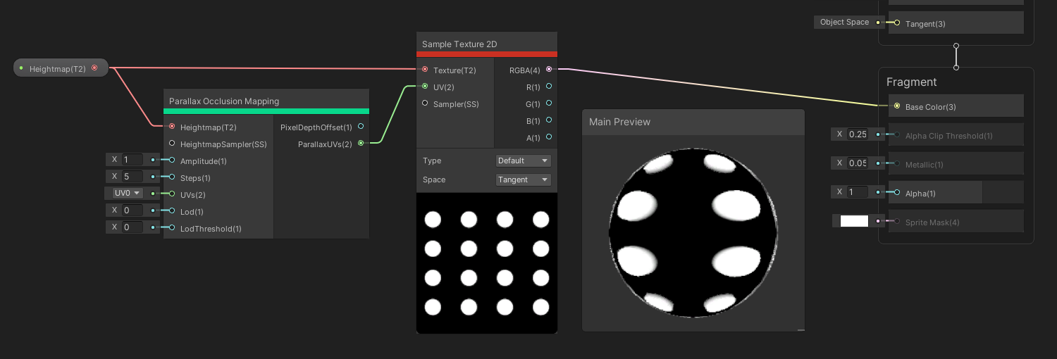Using the same texture for the base and the heightmap, you can see how the offset is applied.

Math Nodes

Math nodes, as you can imagine, are all about basic math operations, ranging from basic arithmetic to vector algebra.

Math/Basic Nodes

₁₀₀ Add

Now we can take a rest with some super simple nodes! I bet you can’t guess what the Add node does. It takes two float inputs, and the output is those two added together.

₁₀₁ Subtract

The Subtract node, on the other hand, takes the A input and subtracts the B input.

₁₀₂ Multiply

The Multiply node takes your two inputs and multiplies them together, although this is more in-depth than other basic maths nodes. If both inputs are floats, they are multiplied together, and if they’re both vectors, it’ll multiply them together element-wise, and return a new vector the same size as the smaller input. If both inputs are matrices, the node will truncate them so that they are the same size and perform matrix multiplication between the two, outputting a new matrix the same size as the smaller input. And if a vector and a matrix are input, the node will add elements to the vector until it is large enough, then multiply the two.

Multiplying is more complex than expected depending on the inputs!

₁₀₃ Divide

The Divide node also takes in two floats and returns the A input divided by the B input.

₁₀₄ Power

The Power node takes in two floats and returns the first input raised to the power of the second input.

₁₀₅ Square Root

And finally, the Square Root node takes in a single float and returns its square root.

Math/Interpolation Nodes

The Interpolation family of nodes are all about smoothing between two values to get a new value.

₁₀₆ Lerp

The Lerp node is extremely versatile. Lerp is short for “linear interpolation” – we take in two inputs, A and B, which can be vectors of up to four components. If you supply vectors of different sizes, Unity will discard the extra channels from the larger one. We also take a T input, which can be the same size as those input vectors, or it can be a single float. T is clamped between 0 and 1. Interpolation draws a straight line between the A and B inputs and picks a point on the line based on T – if T is 0.25, the point is 25% between A and B, for example. If T has more than one component, the interpolation is applied per-component, but if it is a single float, then that same value is used for each of A and B’s components. The output is the value that got picked.

₁₀₇ Inverse Lerp

The Inverse Lerp node does the inverse process to Lerp. Given input values A, B and T, Inverse Lerp will work out what interpolation factor between 0 and 1 would have been required in a Lerp node to output T. I hope that makes sense!

The Lerp result is 25% between 0 and 0.5. The Inverse Lerp result is 0.25.

₁₀₈ Smoothstep

Smoothstep is a special sigmoid function which can be used for creating a smooth but swift gradient when an input value crosses some threshold. The In parameter is your input value. The node takes two Edge parameters, which determine the lower and higher threshold values for the curve. When In is lower than Edge 1, the output is 0, and when In is above Edge 2, the output is 1. Between those thresholds, the output is a smooth curve between 0 and 1.

Smoothstep is great for setting up thresholds with small amounts of blending.

Math/Range Nodes

The Range node family contains several nodes for modifying or working with the range between two values.

₁₀₉ Clamp

The Clamp node takes in an input vector of up to four elements, and will clamp the values element-wise so that they never fall below the Min input and are never above the Max input. The output is the vector after clamping.

Clamp is an easy way to remove values too high or too low for your needs.

₁₁₀ Saturate

The Saturate node is like a Clamp node, except the min and max values are always 0 and 1.

₁₁₁ Minimum

The Minimum node takes in two vector inputs and outputs a vector of the same size where each element takes the lowest value from the corresponding elements on the two inputs. If you input two floats, it just takes the lower one.

₁₁₂ Maximum

And the Maximum node does a similar thing, except it returns the higher number for each component of the input vectors.

₁₁₃ One Minus

The One Minus node takes each component of the input vector and returns one, minus that value. Shocking, I know.

It’s difficult to make these nodes look interesting in screenshots!

₁₁₄ Remap

The Remap node is a special type of interpolation. We take an input vector of up to four elements. Then we take two Vector 2 inputs: one is the In Min Max vector which specifies the minimum and maximum values that the input should have. The Out Min Max vector specifies the minimum and maximum value the output should have. So this node ends up, essentially, performing an Inverse Lerp with the input value and In Min Max to determine the interpolation factor, then does a Lerp using that interpolation factor between the Out Min Max values. The results are then output.

The In input to the Remap is the same as the T input to the Inverse Lerp on this pair of nodes.

₁₁₅ Random Range

The Random Range node can be used to generate pseudo-random numbers between the Min and Max input floats. We specify a Vector 2 to use as the input seed value, and then a single float is output. This node is great for generating random noise, but since we specify the seed, you can use the position of, for example, fragments in object space so that your output values stay consistent between frames. Or you could use time as an input to randomise values between frames.

The Random Range node gives random values depending on an input seed.

₁₁₆ Fraction

The Fraction node takes an input vector, and for each component, returns a new vector where each value takes the portion after the decimal point. The output, therefore, is always between 0 and 1.

This pair of nodes will rise from 0 to 1 then blink right back to 0 continually.

Math/Round Nodes

The Round node family is all about snapping values to some other value.

₁₁₇ Floor

The Floor node takes a vector as input, and for each component, returns the largest whole number lower or equal to that value.

₁₁₈ Ceiling

The Ceiling node is similar, except it takes the next whole number greater than or equal to the input.

₁₁₉ Round

And the Round node is also similar, except it rounds up or down to the nearest whole number.

₁₂₀ Sign

The Sign node takes in a vector and for each component, returns 1 if the value is greater than zero, 0 if it is zero, and -1 if it is below zero.

₁₂₁ Step

The Step node is a very useful function that takes in an input called In, and if that is below the Edge input, the output is 0. Else, if In is above the Edge input, the output becomes 1. If a vector input is used, it operates per-element.

Use Step as a threshold on a color or other value.

₁₂₂ Truncate

The Truncate node takes an input float and removes the fractional part. It seemingly works the same as Floor, except it works differently on negative numbers. For instance, -0.3 will floor to -1, but it truncates to 0.

Math/Wave Nodes

The Wave node family is a very handy group of nodes used for generating different kinds of waves, which are great for creating different patterns for materials.

₁₂₃ Noise Sine Wave

The Noise Sine Wave node will return the sine of the input value, but will apply a small pseudorandom noise to the value. The size of the noise is random between the min and max values specified in the Min Max Vector 2. The output is just the sine wave value.

The noise component adds variation to the usual sine wave.

₁₂₄ Square Wave

A Square Wave is one that constantly switches between the values -1 and 1 at a regular interval. The Square Wave node takes in an input value and returns a square wave using that as the time parameter. If you connect a Time node, then it will complete a cycle each second.

Don’t be square, use the Square Wave today!

₁₂₅ Triangle Wave

A Triangle Wave rises from -1 to 1 linearly, then falls back to -1 linearly. The curve looks like a series of triangular peaks, hence the name. This node goes from -1 to 1 to -1 again over an interval of one second.

Use a triangle wave if you need something sharper than a sine wave.

₁₂₆ Sawtooth Wave

A Sawtooth Wave rises -1 to 1 linearly, then instantaneously drops back down to -1. The curve looks like a series of sharp peaks, like a saw. This node completes one cycle of going from -1 to 1 within a second.

A sawtooth wave is similar to a Time and Modulo combo, but it goes from -1 to 1 instead of 0 to 1.

These four nodes are great for looping material animations over time.

Math/Trigonometry Nodes

The Trigonometry node family invokes fear in the hearts of school students everywhere. If you ever wondered when you’ll ever use trig in later life, this is where.

₁₂₇ Sine, ₁₂₈ Cosine, ₁₂₉ Tangent

The Sine, Cosine and Tangent nodes perform the corresponding basic trig function on the input, which is an angle in radians. Sine and Cosine return values between -1 and 1, where Tangent may return values from -Infinity to Infinity. Sine and cosine functions are used under the hood during cross product calculations.

₁₃₀ Arcsine, ₁₃₁ Arccosine, ₁₃₂ Arctangent

The Arcsine, Arccosine and Arctangent nodes do the opposite - these are the inverse trig functions, and we can use them to get back the angle from our input value (where the input is a valid output value from one of Sine, Cosine or Tangent). All the outputs are in radians: Arcsine accepts values between -1 and 1 and will return an angle between minus pi over 2 and pi over 2; Arccosine accepts inputs from -1 to 1, but this time returns the angle between 0 and pi; and the Arctangent node takes any Float value as input and returns an angle between minus pi over 2 and pi over 2, like Sine.

₁₃₃ Arctangent2

Arctangent2 is the two-argument arctangent function. Given inputs A and B, it gives the angle between the x-axis of a two-dimensional plane and the point vector (B, A).

₁₃₄ Degrees To Radians

The Degrees To Radians node takes whatever the input float is, assumes it’s in degrees, and multiplies it by a constant such that the output is the same angle in radians.

₁₃₅ Radians To Degrees

The Radians To Degrees node does the opposite of Degrees To Radians - give it a radian value, and it’ll return the equivalent value in degrees.

₁₃₆ Hyperbolic Sine, ₁₃₇ Hyperbolic Cosine, ₁₃₈ Hyperbolic Tangent

And finally, the Hyperbolic Sine, Hyperbolic Cosine and Hyperbolic Tangent nodes perform the three hyperbolic trig functions on your input angle. The inputs and outputs are Float values.

It’s not easy to represent these nodes in screenshots.

Math/Vector Nodes

The following Vector nodes can do several basic linear algebra operations for us.

₁₃₉ Distance

The Distance node takes in two vectors and returns, as a float, the Euclidean distance between the two vectors. That’s the straight-line distance between the two.

I think we need a bit of distance.

₁₄₀ Dot Product

The Dot Product is a measure of the angle between two vectors. When two vectors are perpendicular, the dot product is zero, and when they are parallel, it is either 1 or minus 1 depending on whether they point in the same or the opposite direction respectively. The dot product node takes in two vectors and returns the dot product between them as a Float.

When the dot product is 0, the two vectors are orthogonal.

₁₄₁ Cross Product

The Cross Product between two vectors returns a third vector which is perpendicular to both. You will probably use the cross product to get directions, so magnitude doesn’t matter as much, but for clarity, the magnitude of the third vector is equal to the magnitude of the two inputs multiplied by the sine of the angle between them. The cross product node performs the cross product on the two inputs, which must be Vector 3s, and outputs a new Vector 3 – the direction is based on the left-hand rule for vectors. In other words, if vector A points up and vector B points right, the output vector points forward.

Are you cross with me?

₁₄₂ Transform

The Transform node can be used to convert from one space to another. The input is a Vector 3 and the output is another Vector 3 after the transform has taken place. The node has two controls on its body which you can use to pick the Space you want to convert from and to – you can pick between many of the spaces we’ve mentioned before: Object, View, World, Tangent and Absolute World. You can also choose the Type with a third control option, which lets you pick between Position and Direction.

₁₄₃ Fresnel Effect

The Fresnel Effect node is another great node which can be used for adding extra lighting to objects at a grazing angle – specifically, it calculates the angle between the surface normal and the view direction. If applied to a sphere, you’ll see light applied to the ‘edge’, which is easy to see on the node preview. The inputs to the node are the surface Normal and View Dir, both of which are Vector 3s assumed to be in world space, and a float called Power, which can be used to sharpen the Fresnel effect. The output is a single float which represents the overall strength of the Fresnel.

Fresnel, also known as rim lighting, adds a glow at grazing angles.

₁₄₄ Reflection

The Reflection node takes in an incident direction vector and a surface normal as the two inputs, and outputs a new vector which is the reflection of the incident vector using the normal vector as the mirror line.

Let’s reflect on the choices that brought us here.

₁₄₅ Projection

The Projection node takes two vectors, A and B, and projects A onto B to create the output vector. What this means is that we end up with a vector parallel to B, but possibly longer or shorter, depending on the length of A.

Make sure vector B is non-zero!

₁₄₆ Rejection

The Rejection node also takes two vectors, A and B, and returns a new vector pointing from the point on B closest to the endpoint of A, to the endpoint of A itself. The rejection vector is perpendicular to B. In fact, the rejection vector is equal to A minus the projection of A onto B.

We can define rejection in terms of projection. Neat!

₁₄₇ Rotate About Axis

The Rotate About Axis node takes a Vector 3 Input and a second Vector 3 representing the Axis to rotate around, as well as a Rotation angle as a float. We also have a control on the node that lets us choose between degrees and radians for the rotation input. The node outputs the original vector rotated around the rotation axis by that amount.

Not to be confused with the Rotation node.

₁₄₈ Sphere Mask

The Sphere Mask takes a Coordinate, a position in any arbitrary space, and a sphere represented by a Centre point and a Radius. If the original position is within the sphere, the output is 1. Else, it is zero. Although, there’s also a Hardness parameter, which is designed to be between 0 and 1, which you can use to smoothen the falloff between 0 and 1 outputs. The higher the hardness parameter, the sharper the transition. If you want it to be a hard border, set it to 1.

Expand this to three dimensions, and you’ve got a sphere mask.

Math/Derivative Nodes

These Derivative nodes evaluate a set of nodes on adjacent pixels and provide a measure of how different the results are between pixels.

₁₄₉ DDX

The DDX node can be used to take a derivative in the x-direction. This works by calculating the input to the node for this pixel and the adjacent horizontal pixel and taking the difference between them. The output is that difference. You can do this without sacrificing efficiency because during the rasterization process, fragments get processed in 2x2 tiles, so it’s very easy for a shader to calculate values on adjacent pixels in this group of tiles.

₁₅₀ DDY

The DDY node does a similar derivative, except vertically. It takes this pixel and the adjacent pixel vertically and returns the difference between their inputs to this node.

₁₅₁ DDXY

And finally, DDXY takes the derivative diagonally by returning the sum of the two derivatives horizontally and vertically. In effect, it’s like adding DDX and DDY on the same input and taking the absolute value. All three derivative nodes are only available in the fragment shader stage. You might use them for something like edge detection by reading the values from Scene Color or Scene Depth and detecting where there’s a massive difference between adjacent pixels.

You get these derivatives with an unexpectedly low overhead.

Math/Matrix Nodes

Use the Matrix node family to create matrices or carry out basic matrix operations.

₁₅₂ Matrix Construction

The Matrix Construction node can be used to create new matrices using vectors. The node has four inputs, each of which is a Vector 4, corresponding to the maximum matrix size of 4x4. The node has a setting to determine whether the inputs are row or column vectors, and three inputs of varying size – so you can use this node to construct a 2x2, 3x3 or 4x4 matrix.

₁₅₃ Matrix Split

The Matrix Split node, on the other hand, takes in a matrix and lets us split the matrix into several vectors. The input matrix can be between 2x2 and 4x4, and the output Vector 4s will be partially filled with zeroes if the matrix is smaller than 4x4. As with the Matrix Construction node, we can choose whether the output vectors are row or column vectors.

₁₅₄ Matrix Determinant

The determinant of a matrix is a common operation in maths, and the Matrix Determinant node calculates it for you. The input is a matrix of any size between 2x2 and 4x4, and the output is its determinant. This can be a bit costly for large matrices, so use it sparingly.

₁₅₅ Matrix Transpose

The Matrix Transpose node reflects the elements of the matrix in its leading diagonal, such that the rows become columns and vice versa. The input and output are both matrices of the same size.

Matrices are just arrays of numbers - and they’re great in combination with vectors.

Math/Advanced Nodes

This group might be called Advanced, but many of these nodes are basic maths operations.

₁₅₆ Absolute

The Absolute node returns the absolute value of the input – in other words, if the input value is negative, the sign becomes positive. The input can be a vector, and if so, the operation is performed to each element. That applies to a lot of these nodes, so sometimes I’ll just mention a float input even if it can take a vector.

₁₅₇ Length

The Length node takes a vector as input and returns its length, which is calculated using Pythagoras’ Theorem.

₁₅₈ Modulo

Modulo arithmetic works by counting up until you reach some value, at which point you start counting from zero again. In other words, the Modulo node gives the remainder after dividing input A by input B.

₁₅₉ Negate

The Negate node flips the sign of the input float.

₁₆₀ Normalize

The Normalize node takes in a vector and returns a new vector pointing in the same direction, but with length 1.

₁₆₁ Posterize

The Posterize node takes in an input value and a step value. This node will clamp the range of the input between 0 and 1 and quantise its value so that it can only take a number of values equal to the number of steps supplied, plus one. For example, if the number of steps is 4, then the output is rounded down to the values 0, 0.25, 0.5, 0.75 or 1.

Posterize doesn’t mean turning it into a poster, but that would’ve been cool too.

₁₆₂ Reciprocal

The Reciprocal node divides one by the input float. We have an option to pick the algorithm used for the calculation – either Default, or Fast, which is less accurate, but good if you’re using Reciprocal a lot.

₁₆₃ Reciprocal Square Root

The Reciprocal Square Root node is similar to Reciprocal, except it calculates 1 divided by the square root of the input. Unlike Reciprocal, there’s no extra option to choose different methods. If you’re interested in a bit of history, the Fast Inverse Square Root method is a famous piece of code, pioneered by John Carmack but discovered earlier, for calculating the reciprocal square root of a number. It’s no longer necessary because this functionality is provided at the instruction set level, but it’s an interesting footnote.

₁₆₄ Exponential

The Exponential node raises a particular number to the power of the float input. We can pick what the base number is by using the Base dropdown, which lets us choose between 2 and e. e is Euler’s number, which is approximately 2.72.

Exponential nodes are quickly growing in popularity.

₁₆₅ Log

The Log node does the opposite process as the Exponential node. If 2 to the power of 4 equals 16, then the log base 2 of 16 equals 4. We take in a float and return its log under a particular base. We can choose the base using the Base drop-down, except now we have the choice of 2, e or 10.

Logarithms do the opposite of exponents. Compare the two highlighted points with those on Exponential!

Artistic Nodes

Artistic nodes usually operate on colors, or individual color channels, or textures.

Artistic/Blend Nodes

₁₆₆ Blend

The Blend node is normally used to blend one color into another. In this case, we pass a base color and a blend color into the node and we blend the Blend input onto the Base in put according to a third input, which is a float called Opacity. When Opacity is 0, the base is unaltered, and when Opacity is 1, the blending is at its strongest. There is also a Mode dropdown which lets us choose the method used for blending – there are a lot of options so I won’t go over every one. The only output is the color after the blending has been completed.

There are plenty of blending options, similar to those found in graphics programs.

Artistic/Filter Nodes

₁₆₇ Dither

Dither is another of my favourite nodes. We use it in screen-space to apply intentional noise in some way – internally, the node defines a neat pattern of noise values which are used as thresholds. The input is a vector of values, and for each element, if its value is below the threshold defined by the dithering pattern, then the output is 0. Otherwise, it’s 1. We also require the Screen Position as input, and we can multiply this to scale the dithering effect.

Dither is one of my favourite nodes - it’s great for fake transparency effects.

Artistic/Mask Nodes

₁₆₈ Color Mask

The Color Mask node takes in an Input color, a Mask Color, and a Range float. If the input color is equal to the mask color, or within the range specified, then the output of the node is 1. Else, it is zero. However, there’s also a Fuzziness input. If we raise this above zero, then there will be a soft transition between 1 and 0 for values on the edge of the range. The output is a single float representing the mask value.

I’ve picked all the yellow parts of this texture.

₁₆₉ Channel Mask

The Channel Mask node takes in a color as input. The Channels option on the node lets us pick any combination of channels. For each one that is selected, this node keeps colors in that channel, but discards color channels that are not picked by setting their values to zero. The output is the masked color.

If you decide you hate the green channel, now you can delete it.

Artistic/Adjustment Nodes

The following Adjustment nodes are used to tweak the properties of colors.

₁₇₀ Hue

The Hue node can be used to offset the hue of whatever color is passed as an input, using the amount specified by the Offset input. This node comes with a toggle between different Modes – for some reason, the documentation lists the options as Degrees and Radians, but on the node the options seem to be Degrees and Normalized. When Degrees is picked, you cycle through the entire range of hues between 0 and 360. And when Normalized is picked, the hue range is covered between an offset of 0 and 1.

Most people would call cycling through hues ‘changing color’.

₁₇₁ Saturation

The Saturation node adjusts the amount of saturation in the input color by whatever amount is passed into the Saturation float input. When the saturation value is 1, the original color’s saturation is left alone, and when it is zero, the output color will have no saturation at all.

Colors get closer to greyscale as saturation decreases to 0.

₁₇₂ Contrast

The Contrast node does a similar thing, except it adjusts the amount of contrast of the input color by whatever amount is used for the Contrast input float.

Increasing contrast creates very vibrant images.

₁₇₃ White Balance

The White Balance node is used for modifying the Tint and Temperature of an input color. Temperature is a bit hard to pin down, but generally speaking, cold colors are more blue and warm colors are more red, so reducing the temperature below 0 makes the color more blue and raising it above 0 makes things redder. Tint, on the other hand, tends to offset a color towards pink or green when it’s increased.

White Balance does strange things to colors.

₁₇₄ Replace Color

The Replace Color node takes a color input, and we can define a color to replace, called From, and a color to replace it with, called To. Whenever the From color appears, it’s replaced with the To color. We also define a float called Range, which means that if any input color is within that range of From, it will also be replaced. And finally, increasing the Fuzziness input means there will be a smooth falloff between the original colors and the To color.

We can swap out a range of colors easily like this.

₁₇₅ Invert Colors

The Invert Colors node takes an input color, and for each channel, returns one minus the channel. This node assumes the input colors are between 0 and 1 for each color channel, so this might act strange for HDR colors with high intensity.

Invert any combination of color channels easily.

₁₇₆ Channel Mixer

The Channel Mixer node takes in a color input, and for each of the red, green and blue color channels, we can remap the amount they contribute to the output color’s red, green and blue channels. We do this by clicking one of the three buttons labelled R, G and B. When one is selected, modifying the sliders, which can run between -2 and 2, changes how much that input channel contributes to the three output channels. For example, if we select R, then make the sliders 0, 0 and 2, that means the input red contributes 200% to the output blue.

In this image, both red and green contribute to output blue, weighted equally.

Artistic/Normal Nodes

The Normal node family is irreplaceable when working with normal mapping, whether you’re reading from a texture or creating the normals within Shader Graph.

₁₇₇ Normal Unpack

The Normal Unpack node takes a color or vector as input and unpacks it into a normal vector. That said, for textures, you can usually sample it as a normal map anyway, so this node is more useful if you’ve generated a normal texture within the graph somehow and you need to convert from colors to normal vectors. You can choose the Space of the input between Tangent or Object space using the dropdown. The output normal vector is a Vector 3.

You can use Normal Unpack, but Sample Texture 2D can do the same thing.

₁₇₈ Normal Strength

The Normal Strength node takes a set of normals as input as a Vector 3 and scales their strength via the Strength float input. A strength of 1 leaves the normals unaltered, while 0 will return a completely flat normal map with all the normals pointing upwards.

If your normals are a bit too strong, we can tone them down a little.

₁₇₉ Normal From Texture

The Normal From Texture node takes a Texture, a Sampler and a set of UVs as input and uses that as a heightmap, from which it will generate normals. The Offset float input defines how far away the normal details extend from the surface, and the Strength float input multiplies the size of the result. The output is a Vector 3 representing the calculated normal vector.

This provides an easy way to convert heightmaps to normals.

₁₈₀ Normal From Height

The Normal From Height node is similar, except it takes in a singular height value and generates a normal vector based on the that and the input Strength float. We can change the Space used for the output normals between Tangent and World. Tangent is useful for working with textures, whereas World is great for working with lighting.

We can generate height data in the shader and convert it to normals like this.

₁₈₁ Normal Blend

The Normal Blend node takes in two normals, adds them together, normalises them and returns the result. This is great for combining a base normal texture, A, and a detail normal texture, B, together. We have the choice of two modes here: Default does what I just described, and Reoriented will rotate the normal by the angle between the first and second map. By doing that, the detail normal texture isn’t just layered on top of the base normal texture – it acts as if the detail normal texture is mapped onto the surface described by the base normal.

Will it blend? Well normally, yes.

₁₈₂ Normal Reconstruct Z

The Normal Reconstruct Z node takes in a generated normal vector as a Vector 2 and calculates what the Z component should be for the output Vector 3.

This lets you package your normal data into the red and green channels of the texture, so long as you know the normals always point in the positive direction, freeing up the blue and alpha channels for other uses to reduce the number of texture samples and texture memory your shader requires. For example, you could include a smoothness map in the blue channel, since it only requires greyscale data, but you’ll need to create these packed textures externally.

We can hide extra data by using only two channels for normal data.

Artistic/Utility Nodes

₁₈₃ Colorspace Conversion

The Colorspace Conversion node can be used to convert an input color between the RGB, HSV and Linear color spaces. We have two dropdown options to pick the Input and Output color spaces.

This makes it easy to work in other color spaces, such as HSV.

Procedural Nodes

₁₈₄ Checkerboard

The Checkerboard node creates an alternating pattern of tiles, colored according to the Color A and Color B inputs. The UV is used for mapping the pattern onto objects and the Frequency Vector 2 is used for scaling the checkboard in those respective axes. The output is the checkerboard color as a Vector 3, although as of this article, the documentation accidentally lists the output as a UV Vector 2.

Checkerboard patterns are great for prototyping especially.

Procedural/Noise Nodes

Noise is one of the best tools to use within shaders if you want to create procedural content or if you want highly customisable properties on your materials.

₁₈₅ Simple Noise

The Simple Noise node generates a basic type of noise pattern called “value noise”, using a UV input to map the noise onto your mesh and a Scale input float to rescale the noise texture in both directions. The output is a single float representing a noise value between 0 and 1.

₁₈₆ Gradient Noise

The Gradient Noise node generates a slightly more sophisticated type of noise called Perlin Noise using the same UV and Scale inputs as Simple Noise, and a single float output once again. Perlin Noise is a very common type of noise used in random generation, particularly for textures and terrains.

₁₈₇ Voronoi

The Voronoi node is a very pretty and versatile type of noise. It works by generating points on a grid, repositioning them in random directions, then coloring each pixel in the grid based on distance from a point – the closer to a point we are, the darker the pixel is. We supply a UV for mapping the texture, plus an Angle Offset float for randomly moving the points and a Cell Density float to decide the number of points that are added. The Out output just gives the distance from the closest point as a float, which is usually used as the Voronoi pattern. The Cells output gives us what Unity calls the “raw cell data”, although reading the autogenerated code in the documentation, it seems to be colored based on the random x offset for each cell.

Noise is your best friend when dealing with procedural materials.

Procedural/Shapes Nodes

The Shapes node family are all Signed Distance Fields, or SDFs, representing different shapes as either white inside the shape, or black outside it.

₁₈₈ Rectangle

The Rectangle node takes an input UV and a Width and Height float, then generates a rectangle with that width and height. The width and height should be between 0 and 1, and if you use the same value for both, you should get a square texture. The output of the node is 1 if the pixel is within the rectangle, and 0 otherwise. These shapes can only be generated in the fragment stage.

₁₈₉ Rounded Rectangle

The Rounded Rectangle node is exactly the same as Rectangle, except it adds a Radius float option to specify how much the corners of the rectangle shape should be rounded.

₁₉₀ Ellipse

The Ellipse node similarly takes a Width and Height float and a UV Vector 2 and will generate an ellipse. If you give it an equal width and height, you’ll end up with a circle.

₁₉₁ Polygon

The Polygon node uses those same Width, Height and UV inputs, and also adds a Sides input which defines how many edges the shape has. The result will be a regular polygon that’s been stretched if the width and height are different.

₁₉₂ Rounded Polygon

And finally, the Rounded Polygon node has the same inputs as Polygon, plus a Roundness float option which acts like the radius option on Rounded Rectangle.

These SDF-based shape nodes give you a good starting point for procedural materials.

Utility Nodes

These Utility nodes are for miscellaneous things, but as it turns out, three of them are extremely powerful nodes which can transform the way your graph fundamentally works… plus the Preview and Redirect nodes.

₁₉₃ Preview

The Preview node takes in a vector input and outputs precisely the same thing. The reason for using this node is that it displays what your shader looks like at this point, so it’s extremely useful for visually debugging your shaders. In previous versions of Shader Graph which didn’t feature Redirect Nodes, which you can add by double-clicking an edge, Preview nodes used to have a secondary use for redirecting edges in particularly messy graphs.

₁₉₄ Redirect

Double-click on any wire between node inputs/outputs and you’ll create a Redirect node between them. It has no effect on the shader output, but you can move the Redirect node around clean up your graph.

Preview doesn’t work on every input - mostly just colors and vectors.

₁₉₅ Keyword

These are listed in their own section in the Create Node menu, but I’ll talk about them here. Whenever you drag a Keyword node onto the graph, which are based on whatever Keyword properties you’ve added, it will have a number of inputs and a single output. Depending on the value of the keyword defined on this material in the Inspector, a keyword node will pick whatever was input to the corresponding keyword option. For example, if we use a Boolean keyword, we can connect a range of nodes to both the On and Off inputs and the output is chosen based on the value of the keyword.

Based on the value of the keyword, the output of the node will change.

₁₉₆ Sub Graph

These are also in a separate section like Keyword nodes. A Sub Graph is a separate kind of Shader Graph we can create. They have their own output nodes, which we can add outputs to, and when we add properties to a sub graph, they become the inputs to the resulting Sub Graph node. Then we can create nodes in the usual way on the graph. Once we’ve created a sub graph, we can search for them in our main graph and use them like any other node – the properties of the sub graph appear as the inputs on the left, and the outputs inside the sub graph appear as the outputs on the right of the node.

Sub Graphs lets us condense lots of nodes into a single node.

₁₉₇ Custom Function

The Custom Function node lets us write custom shader code to run inside the node. I won’t go into detail here because this node is probably one of the most complicated and bespoke of them all, but if we click on the Node Settings, we can define a list of inputs and outputs of whatever types we like, and then we can attach a shader code file or write code directly into the settings window. That custom code is written in HLSL and we can write the name of the specific function from the file to use for this node.

A common operation with custom function nodes is to get information from lights in the scene.

Utility/Logic Nodes

As a palate cleanser, we can deal with some Boolean logic nodes.

₁₉₈ And

The And node takes two Boolean values which can be true or false, 1 or 0. If they are both true, or 1, then this node returns true. Else, the node returns false.

₁₉₉ Or

The Or node also takes two Boolean inputs. If either or both of them is true, then the node outputs true. Else, it outputs false.

₂₀₀ Not

The Not node takes a single input and returns the opposite value. In other words, if true is input, false is output.

₂₀₁ Nand

The Nand node is equivalent to doing And, then passing the result into a Not node. If both inputs are true, the output is false. Else the output is true. At least, in theory - the actual outputs of this node seem to act like a Nor operation, not Nand. Strange.

₂₀₂ All

The All node takes in a vector of values. If every element is non-zero, the output of the node is true.

₂₀₃ Any

On the other hand, the Any node also takes in a vector, and returns true if any of the input elements are non-zero.

₂₀₄ Comparison

The Comparison node is used to compare the values of two input floats. Based on the Comparison operator chosen from the dropdown in the middle of the node, a Boolean value is output. Those operations are Equal, Not Equal, Less, Less Or Equal, Greater, Greater Or Equal. For instance, if the two inputs are 7 and 5 and your operation is Greater, then the output is True.

₂₀₅ Branch

The Branch node can be used to take decisions in your shader, similar to an if-statement in C#. If the Input predicate is true, this node takes the value of whatever is plugged into the True input. Otherwise, it outputs whatever is in the False input. Beware that both sides will be fully calculated and the invalid branch is discarded, so it’s not a good idea to have huge node trees plugged into both True and False. If possible, move this check as early on in the graph as you can to minimise the size of the node tree plugged into both sides.

₂₀₆ Is NaN

The Is NaN node is shorts for “Is not a number”. In floating-point arithmetic, NaN is a special value representing an invalid number. This node returns true if the input float is NaN, and false otherwise.

₂₀₇ Is Infinite

Similarly, Infinite is a special value that floating points can take. The Is Infinite node returns true if the input is infinite.

₂₀₈ Is Front Face

A mesh defines whether faces are front-facing or back-facing based on the winding order of its vertices. That means the order the vertices are listed in the mesh data. The Is Front Face node will always return true unless the Two Sided option is ticked in the Graph Settings. But when it is ticked, we can decide to change the behaviour of the shader based on the facing direction of the mesh.

There’s a lot of logic-based nodes - not much else accepts a Boolean.

Conclusion

And that’s every node covered! Shader Graph is an amazing visual tool for building shaders, and while it doesn’t yet cover every use case for shaders – most notably, it’s missing support for tessellation and geometry shaders, as well as stencils – the sheer number of nodes included out of the box make it a fantastic inclusion for Unity.

This article took a long time to put together, as did the YouTube video version, so thanks for reading and watching. If you enjoyed this or learned something, I’d appreciate you checking out my YouTube. The same content gets posted there as on my website, and I need as much support as I can to grow both! And check out my Patreon – there’s a bunch of goodies up for grabs for subscribers. Until next time, have fun making shaders!

Acknowledgements

Supporters

Support me on Patreon or buy me a coffee on Ko-fi for PDF versions of each article and to access certain articles early! Some tiers also get early access to my YouTube videos or even copies of my asset packs!

Special thanks to my Patreon backers for May 2021!

Gemma Louise Ilett
JP $\cdot$ Pablo Ruiz
Jack Dixon $\cdot$ Paul Froggatt $\cdot$ Tuomas Männistö $\cdot$ Sébastien Perouffe
Chris Sims $\cdot$ FonzoUA $\cdot$ Josh Swanson $\cdot$ MR MD HARDING $\cdot$ Moishi Rand $\cdot$ Shaun Wall
Anna Voronova $\cdot$ Christopher Pereira $\cdot$ Harshad $\cdot$ James Poole $\cdot$ Lee Miller $\cdot$ Ming Lei $\cdot$ Zachary Alstadt

And a shout-out to my top Ko-fi supporters!

Hung Hoang $\cdot$ Arthur H $\cdot$ Megan Taylor $\cdot$ Takuya $\cdot$ “Somebody”